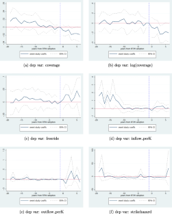
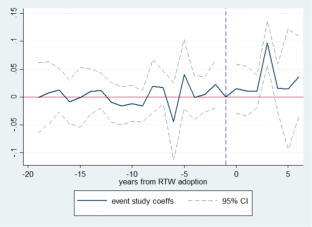
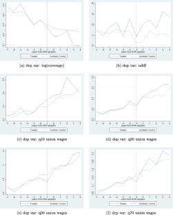
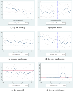
Right-to-work (RTW) laws prohibit union security agreements in many U.S. states, and are frequently portrayed as a mortal threat to unionism in the country. This paper sheds new light on the old debate surrounding the effects of RTW legislation by evaluating their impacts in six U.S. states that adopted such laws in the 21 st century. Using a mix of panel data methods, I find evidence that in the private sector, RTW laws decrease union coverage by more than 10 percent, all else equal. I find RTW laws to have only a small and insignificant effect on free-riding behavior as measured by the share of unionized workers who are nonmembers. Union formation through NLRB-administered elections do not appear to be adversely affected. RTW laws are also found to increase union wages and their premium over non-union wages, which plausibly reflect changes in union bargaining behavior. In the public sector, RTW laws are associated with declines in union coverage but may be confounded by other state-level policies aimed at weakening public sector unions. Separately evaluating the effects of the 2018 U.S. Supreme Court decision in Janus v. AFSCME, which effectively made the entire U.S. public sector right-to-work, I find no evidence of any impact on union-related outcomes. Some of these findings are quite novel, and challenge conventional assumptions about how RTW laws impact unions.
This is a preview of subscription content, log in via an institution to check access.
Price includes VAT (France)
Instant access to the full article PDF.
Rent this article via DeepDyve
The datasets generated during and/or analysed during the current study are available in the Open ICPSR repository, at https://www.openicpsr.org/openicpsr/project/141581/version/V1/view.
Stata codes available from the author upon request.
A typical argument along this line can be found in Shermer, Elizabeth Tandy (2018, April 24) The right to work really means the right to work for less, The Washington Post. https://www.washingtonpost.com/news/made-by-history/wp/2018/04/24/the-right-to-work-really-means-the-right-to-work-for-less/(accessed October 12, 2020). Also see Neal, Candy (2012, January 13) Local union opposes right-to-work movement, The Herald https://duboiscountyherald.com/b/local-union-opposes-right-to-work-movement(accessed May 12, 2021) for a sampling of how union activists view the issue.
This cost is non-trivial: as documented by Bennett (1991), annual dues and fees collected by unions amounted to $504 (current dollars) per union member in 1987.
Taft-Hartley did allow union-shop agreements (unless banned by RTW laws), which technically did require new hires to become union members within some prescribed period as a condition of employment, but a court decision in the 1951 Union Starch Refining v. National Labor Relations Board case made union-shop clauses practically unenforceable (Cogen 1954).
The share of nonmembers does not necessarily have to rise to bring about this outcome, if the share of nonmembers is large to begin with: the loss of agency fee revenue from existing nonmembers alone could be enough to reduce the supply and demand for unions. But this is not very likely given the low percentage of covered nonmembers in non-RTW states.
Lafer (2013) makes a similar claim regarding many anti-labor policies pursued by the same cohort of Republican state governments, such as restrictions on public sector collective bargaining – they bore no relation to local conditions such as levels of state and local government debt
Note that such nonmembers would only be free-riders in the true sense under an RTW regime; in non-RTW states they are at worst ‘cheap riders’ given that they do pay agency fees, which are usually cheaper than full membership dues (Swindle 1984).
Specifically, I performed Shapiro-Wilk tests for the normality of residuals after regressing each dependent variable in level and log forms (controlling for economic and political variables) and chose the specification that yielded a W statistic closer to 1. Due to the high power of the Shapiro-Wilk test, normality was rejected at the 1 percent level for all residuals expect for those pertaining to log(freeride) and log(duration). When histograms of residuals are plotted, those pertaining to coverage, freeride, and duration have obviously right-skewed distributions; the rest have distributions that are at least roughly symmetric.
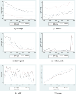
Coverage in the treatment states stood at an average of 9 percent on the eve of RTW legislationNote that inflows to the stock of unionized workers does not strictly equal inflows to the stock of workers covered by union contracts (which the variable ‘coverage’ measures): newborn unions still have to win a collective bargaining agreement.
Springer Nature remains neutral with regard to jurisdictional claims in published maps and institutional affiliations.
This section describes in detail how I constructed each of the variables used in my analyses. Note that some of the variables described here do not appear in the main text, as they are only used as inputs in the construction of our variables.
All CPS-based variables except ‘popul’, ‘emp’, ‘unemp’, and ‘manuf’ have been computed separately for the private and public sector. I have excluded federal government employees in computing the public sector variables. All variables are computed from the CPS Merged Outgoing Rotation Groups (MORG) files released by the National Bureau of Economic Research (NBER), available for download at https://www.nber.org/research/data/current-population-survey-cps-merged-outgoing-rotation-group-earnings-data; the Earner Study weights (‘earnwt’) are used for all aggregation and estimation purposes.
‘popul’: this is the total population of a state in a given year, used as denominator for per-capita variables. This is obtained by summing the individual weights in each state-year cell and dividing by 12.
‘emp’: share of persons aged between 16 and 64 who are currently employed (including self-employed) and at work.
‘unemp’: share of those looking for work or on layoff (unemployed) among a workforce defined as all wage and salary workers plus the unemployed.
‘manuf’: share of wage and salary workers whose industry code ‘dind’ (an NBER-created two-digit industry classification code) is between 5 and 28 in years prior to 2000 and ‘dind02’ is between 5 and 20 for 2000 onward.
‘coverage’: share of employed (private- or public-sector) wage and salary workers who report being either a union member or covered by a union contract.
‘freeride’: share of workers covered by union contracts who report not being a union member.
‘uwage’: weighted average hourly earnings (in nominal dollars) of wage and salary workers covered by union contracts. For workers not paid on an hourly basis, this is usual weekly earning at the main job divided by usual hours worked per week at the main job. I drop observations of over USD 200 per hour, as these are most likely mismeasured. Also dropped are all imputed earnings.
‘nuwage’: the non-union counterpart to ‘uwage’.
‘udiff’: union wage differential estimated for each state×year cell, or \(\hat \) in the wage regression:
$$lwage_=\alpha+\beta union_+X_ +\epsilon_,$$where i indexes workers, lwage is logged hourly wage, union is the union coverage indicator, X is a vector of worker and job attributes (age, age squared, educational attainment, sex, marital status, black, part-time status, whether paid by the hour, dummies for two-digit industry and occupation codes), and 𝜖 is an error term. A well-known source of bias in estimating the union wage differential using CPS data is that earnings for individuals who do not report them are imputed based on the earnings of comparable workers without accounting for their unionization status: this results in attenuation bias for estimating the union wage differential (Hirsch and Schumacher 2004). To address this, I remove all observations with allocated (imputed) earnings for estimating the wage equation.
These variables are also disaggregated by sector (private and public). They are based on the US Bureau of Labor Statistics (BLS)’s Work Stoppages tables (Detailed Monthly Listing, 1993-Present) available at https://www.bls.gov/wsp/ and the US Federal Mediation and Conciliation Service (FMCS)’s work stoppages tables (which had been previously available in Excel format at https://www.fmcs.gov/resources/documents-and-data/). The BLS data records all strikes involving more than 1,000 workers; the FMCS data records all smaller strikes. Unlike the BLS tables, the FMCS tables do not classify struck establishments by ownership status (government or private industry). To identify public sector strikes in FMCS records, I looked for employer names containing the strings ”school”, ”unified school district”, ”USD”, ”U.S.D.”, ”university of”, ”government”, ”authority”, ”of education”, ”state of”, ”county”, and ”municipal”.
‘counts’: number of work stoppages in each state that began in a calendar year and lasted no longer than half a year. Strikes that are missing end dates, and all ongoing strikes as of the end of 2019 are excluded, as are strikes classified as ”interstate”.
‘idled’: annual number of workers involved in all strikes (that are not excluded in ‘counts’) in a given state.
‘strikehazard’: ‘idled’ times 1,000 divided by the number of unionized workers estimated from CPS data.
‘duration’: \(\frac _ n_\cdot d_\) , where ni =number of workers idled in strike i, N = Σini, and di=duration of strike i measured in business days. The FMCS did not record di, so I calculated the total number of days (including weekends) a strike lasted based on its beginning and end dates, and multiplied by \(\frac \) . Some state-year cells are missing duration values because no strike was observed in those cells: it is difficult to say how long a strike would have lasted had there been one.
Up to year 2017, these variables are constructed using a dataset on NLRB elections compiled by Zachary Schaller in Schaller (2019), who generously shared it with me for use in this paper. For years 2018 and 2019, I constructed the same variables using NLRB’s annual election reports (in PDF format) available at: https://www.nlrb.gov/reports/agency-performance/election-reports.
‘cert’: number of union certification elections (identified by a dummy variable for RC petitions) where the percentage of votes in favor (‘pct_for’) is greater than 0.5.
‘decert’: number of de-certification elections (RD petitions filed by employees and RM petitions filed by employers) where ‘pct_for’ is below 0.5.
‘inflow’: total number of eligible employees in certification elections won by unions.
‘outflow’: total number of eligible employees in de-certification elections lost by unions.
‘inflow_perK’: ‘inflow’ times 1,000 divided by the number of non-union workers.
‘outflow_perK’: ‘outflow’ times 1,000 divided by the number of unionized workers.
‘lgdp’: log of annual state per-capita GDP. Gross nominal state GDP is obtained from the U.S. Bureau of Economic Analysis’ Series SAGDP1; this is then divided by ‘popul’ to generate per-capita GDP.
‘Dgdp’: first-differenced ‘lgdp’.
‘jcr_birth’: percentage of private sector employment due to newly created establishments, taken from the US Census Bureau’s Business Dynamics Statistics (BDS_ variable ‘job_creation_rate_birth’. The dataset is available at https://www.census.gov/data/datasets/time-series/econ/bds/bds-datasets.html.
‘jdr_death’: percentage of private sector employment lost due to establishment closures. Same source as ‘jcr_birth’, BDS variable name ‘job_destruction_rate_death’.